Selected Publications

Given two graphs, the graph matching problem is to align the two vertex sets so as to minimize the number of adjacency disagreements between the two graphs. The seeded graph matching problem is the graph matching problem when we are first given a partial alignment that we are tasked with completing. In this paper, we modify the state-of-the-art approximate graph matching algorithm *FAQ* of Vogelstein et al. (2015) to make it a fast approximate seeded graph matching algorithm, adapt its applicability to include graphs with differently sized vertex sets, and extend the algorithm so as to provide, for each individual vertex, a nomination list of likely matches. We demonstrate the effectiveness of our algorithm via simulation and real data experiments; indeed, knowledge of even a few seeds can be extremely effective when our seeded graph matching algorithm is used to recover a naturally existing alignment that is only partially observed.
PR

In various data settings, it is necessary to compare observations from disparate data sources. We assume the data is in the dissimilarity representation (Pękalska and Duin, 2005) and investigate a joint embedding method (Priebe et al., 2013) that results in a commensurate representation of disparate dissimilarities. We further assume that there are “matched” observations from different conditions which can be considered to be highly similar, for the sake of inference. The joint embedding results in the joint optimization of fidelity (preservation of within-condition dissimilarities) and commensurability (preservation of between-condition dissimilarities between matched observations). We show that the tradeoff between these two criteria can be made explicit using weighted raw stress as the objective function for multidimensional scaling. In our investigations, we use a weight parameter, w, to control the tradeoff, and choose match detection as the inference task. Our results show weights that are optimal (with respect to the inference task) are different than equal weights for commensurability and fidelity and the proposed weighted embedding scheme provides significant improvements in statistical power.
In JoC

In this thesis, we investigate how to perform inference in settings in which the data consist of different modalities or views. For effective learning utilizing the information available, data fusion that considers all views of these multiview data settings is needed. We also require dimensionality reduction to address the problems associated with high dimensionality, or “the curse of dimensionality.” We are interested in the type of information that is available in the multiview data that is essential for the inference task. We also seek to determine the principles to be used throughout the dimensionality reduction and data fusion steps to provide acceptable task performance. Our research focuses on exploring how these queries and their solutions are relevant to particular data problems of interest.

Infrared (IR) imaging has the potential to enable more robust action recognition systems compared to visible spectrum cameras due to lower sensitivity to lighting conditions and appearance variability. While the action recognition task on videos collected from visible spectrum imaging has received much attention, action recognition in IR videos is significantly less explored. Our objective is to exploit imaging data in this modality for the action recognition task. In this work, we propose a novel two-stream 3D convolutional neural network (CNN) architecture by introducing the discriminative code layer and the corresponding discriminative code loss function. The proposed network processes IR image and the IR-based optical flow field sequences. We pretrain the 3D CNN model on the visible spectrum Sports-1M action dataset and finetune it on the Infrared Action Recognition (InfAR) dataset. To our best knowledge, this is the first application of the 3D CNN to action recognition in the IR domain. We conduct an elaborate analysis of different fusion schemes (weighted average, single and double-layer neural nets) applied to different 3D CNN outputs. Experimental results demonstrate that our approach can achieve state-of-the-art average precision (AP) performances on the InfAR dataset:(1) the proposed two-stream 3D CNN achieves the best reported 77.5% AP, and (2) our 3D CNN model applied to the optical flow fields achieves the best reported single stream 75.42% AP.
Proc. CVPR

We present a novel approximate graph matching algorithm that incorporates seeded data into the graph matching paradigm. Our Joint Optimization of Fidelity and Commensurability (JOFC) algorithm embeds two graphs into a common Euclidean space where the matching inference task can be performed. Through real and simulated data examples, we demonstrate the versatility of our algorithm in matching graphs with various characteristics--weightedness, directedness, loopiness, many-to-one and many-to-many matchings, and soft seedings.
In arxiv

Recent Publications

Software

RGraphM is a graph matching R package based on [graphm]http://cbio.mines-paristech.fr/graphm/. Coming soon to CRAN.

Recent & Upcoming Talks

Recent Posts

Part of my dissertation research was on the graph matching problem. For solving this problem in real settings, it is useful to think of vertices as elements of a space with the edges determining some sort of locality, (I guess this can be formalized with topology ). Then the graph/vertex matching problem becomes sort of a point cloud matching problem where you don’t know where the points are , just the neighborhood relationships between them ( several manifold learning uses these relationships to find the manifolds defined by the points ).

CONTINUE READING

I have decided to switch to the academic theme for hugo , as it makes much more sense for a researcher. Now I just need to collect all the things I have done over the years.

CONTINUE READING

Content can be written using Markdown, LaTeX math, and Hugo Shortcodes. Additionally, HTML may be used for advanced formatting.

CONTINUE READING

I have been trying to build an R package that uses C code. I was not fast enough to get a working build for some time as it is a wrapper package around an existing C library and I wanted to submit to CRAN eventually, so I needed to get a linux and windows (32 and 64-bit) builds working correctly. Building an R package even with native R code is not easy.

CONTINUE READING

I am in the process of creating my new personal website. I wanted to make it simple and based on a simple design with the option to generate pages without messing with HTML. That is why I am using Herring Cove. This may be overkill for a personal website.

CONTINUE READING

Projects

Some of the things I have worked on.

ALADDIN

ALADDIN : Automated Low-Level Analysis and Description of Diverse Intelligence Video

CVRG

Prediction of Heart Arrythmias

Data Fusion from Disparate Dissimilarities and Joint Optimization of Fidelity and Commensurability

My thesis project. How to use disparate data with very different representations for inference purposes

External Project

An example of linking directly to an external project website using external_link.

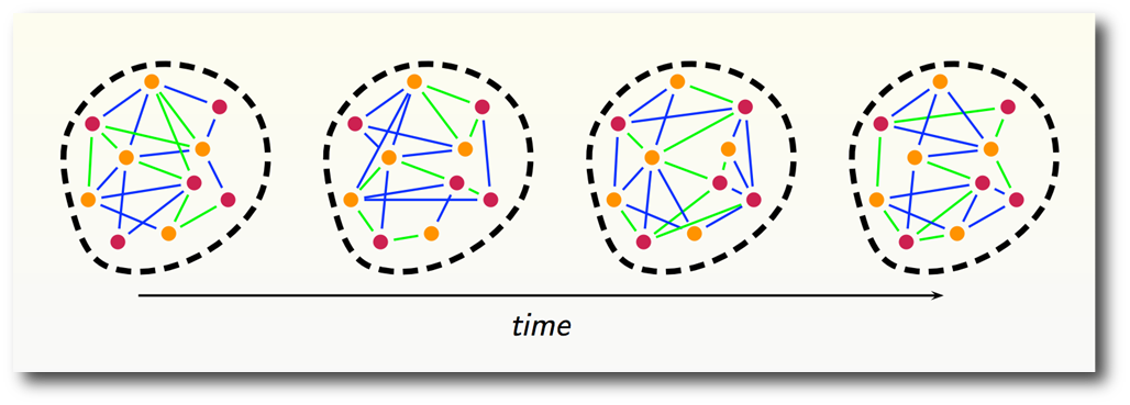
Seeded Graph Matching

The other portion of my disseration project.

XDATA

DARPA program for organizing big data analysis and visualization efforts.

Teaching

I taught an intersession course on R programming at Johns Hopkins. Here are my class notes:

Let’s first start Rstudio. This is a good GUI that helps you organize the R expressions(functions called with some arguments) you run, the plots and outputs as a result of those commands.

We have four panes. The upper left is the R script file editor, where you will enter your commands and save them as a text file. The lower left is the R console where you will see the commands sent to R and the results of those expressions. The results of expressions can be stored in variables to be used in future expressions. The upper right shows the variables and the data stored in those variables. The lower right pane has Files,Plots,Packages,Help tabs. -Files will list the files in the current working directory in your computer’s file system -Plots will show you any plots you have asked R to draw. -Help is where you can see information about R functions -Packages: we don’t need to worry about now

We’ll use R to read, modify and analyze data. Let’s start entering some R expressions and see the results.

How to store data in R

The most basic way one can think of to organize numeric data is a vector. Let’s create a vector whose elements are numbers by concatenating a few of them. We’ll call “c” function with the numbers as arguments to the function.

#creating a numeric vector
a.vector <- c(2,4,5)

If we need a sequence of integers, we can use double colon operator between the starting integer and ending integer

another.vector <- 2:6

We can concatenate different vectors to get new vectors. a.brand.new.vector <-c(a.vector,another.vector)

For any sequence with regular increments, “seq” is the function to use. It has three arguments the first number , the last number and the interval

a.seq.of.numbers <- seq(0,1,0.01)

If we need to store data as a two-dimensional array , we use “array” function (with number of rows and columns)

an.array <- array(a.seq.of.numbers,dim=c(10,10))

In the “array” function, we make use of the “dim” argument which is a vector of length two(number of rows and number of columns). Note that the functions we call might have possible arguments that we don’t provide. R will assume the values of those arguments are the default values, which you can look up in the help document for that function. To do that, enter

?array

We usually won’t need to look up all these arguments, though, since the default values are sensible.

day.number <- 1:7

What is the size of the vector?

length(day.number)

Suppose the data is not numeric, but is composed of strings(any combination of characters words, sentences, etc.) ( Qualitative data for example). We can store multiple strings in a vector like numbers. We call such vectors “character vectors”. We let R know we’re dealing with characters by putting quotes around them.

#Creating a character vector

#We can store qualitative data as vectors, too. (2.1.1)
day.names <- c("Mon","Tue","Wed","Thu","Fri")

During analysis of data, one often needs to modify some portion of a vector. we use square brackets after the name of the vector and inside the brackets we enter a vector of indices. The elements are indexed starting from 1 so if we want to get the first three elements of “day.names”

# If we want to use only part of a vector, we use indexing to choose
# which elements want
#Numeric indexing
day.names[1:3]

If we want to get the elements with indices 2,4,5 (the numbers we had stored in a.vector

day.names[a.vector]

When we need to access some portion of the two-dimensional array we created

an.array[1:4,1:3]

If we want to edit some elements of vectors and arrays, we can edit them in RStudio. If you’re using Rgui, we can use edit function to open up a spreadsheet interface

edit(an.array)

An array is a two-dimensional array of numbers or strings. But data can be a combination of different kinds of variables. The traditional convention of data organization in spreadsheet format is columns corresponding to different variables or features (qualitative or quantitative) being studied and rows corresponding to different observations of those variables. We will use data frames in R to store data organized like this. A data frame in R is a collection of vectors that all have the same length, but can be of any type (numeric vector, character vector). Each vector forms one column of the data frame. Many datasets that you load into R will be stored in data frames.

# data.frames in R

Let’s create a data.frame that is composed of the name of days and the integer corresponding to that day. “data.frame” function creates a data frame with each supplied argument as one of the columns. Columns can also be named, the names of the columns are supplied when creating the data frame. In the following example, these are “number” and “names” respectively

#creating a data.frame (many datasets will be in this form)
a.data.frame <- data.frame(number=day.number,names=day.names)

This R expression caused an error, because we didn’t have vectors that have the same length. Let’s fix this

day.names <- c(day.names,"Sat","Sun")

a.data.frame <- data.frame(number=day.number,names=day.names)

The indexing for data.frames is like arrays:

#Indexing for data frames
a.data.frame[1:3,]
a.data.frame[,2]

One can also access specific columns by using the name of that column, which will return the vector in that column

a.data.frame$names

And we can access some portion of that vector like any vector

a.data.frame$names[1:3]

The variables in data can also be logical variables, that is they take one of the values TRUE or FALSE. Logical vectors that store this kind of data are very useful, especially in indexing.

# A vector can be composed of logical values, too(TRUE or FALSE)
a.logic.vector<-c(TRUE,FALSE,TRUE,FALSE,FALSE,FALSE,FALSE)

If we use one of the comparison operators (“<”,”>”,”<=”,”>=”,”==”) with other type of vector, the result will be a logical vector whose elements are TRUE or FALSE. The value in the logical vector will be TRUE, when the comparison is true.

day.names==”Mon”
day.names==”Tuesday”
day.number<3

If we wanted to get some specific elements of a vector, say “a”, we can use logical vectors that have the same length as index vectors to extract those specific elements. The elements of “a” that will be extracted are the ones which have TRUE values in the logical vector used for indexing

#logical indexing (3.3,3.4)
day.names[a.logic.vector]

# Count the number of TRUEs in the logical vector
sum(a.logic.vector)

The logical indexing is very useful, when you want to extract some portion of the vector that satisfies a particular condition. Let’s look at an example

This function will load a dataset that’s built into R. This dataset includes a vector with the name nhtemp. It will be loaded with the name nhtemp. It’s the yearly temperature record from New Haven.

data(nhtemp)

One can use ls() function to list all the variables that are currently loaded into R

ls()

nhtemp is an R variable that’s slightly different than a vector, so we first want to turn into a regular vector.

nhtemp <- as.vector(nhtemp)

If we want to get temperature records that are higher than 54 degrees, we can use the logical vector

nhtemp>54
nhtemp[nhtemp>54]

If we want to get the indices of the TRUE values in logical vectors, we use the “which” function

which(nhtemp>54)

Now we can use plot functions to plot this series of tempearatures If we use only one argument in the plot function,

plot(nhtemp)

If we want to plot x-y plot (temperature against the years

plot(1912:1971,nhtemp)

plot(1:60,nhtemp,type='l')

These are the summary statistics functions in R

mean(nhtemp)
median(nhtemp)
max(nhtemp)
min(nhtemp)
var(nhtemp)

sd(nhtemp)
sqrt(var(nhtemp))
summary(nhtemp)

For plotting histograms, we use hist function with different

hist(nhtemp)
hist(nhtemp,breaks=14)
hist(nhtemp,breaks=seq(min(nhtemp),max(nhtemp),0.5))
boxplot(nhtemp)
smokes = c("Y","N","N","Y","N","Y","Y","Y","N","Y")
amount = c(1,2,2,3,3,1,2,1,3,2)

a.table <- table(smokes,amount)
prop.table(a.table)

chisq.test(a.table)

Contact